Regression models are incredibly powerful and can save you heaps of time trawling through your data. However, unless you are a trained statistician,  you might be not so confident in using it.  

How to make predictions and interpret the variables? How to assess the quality of the model, and how to diagnose assumptions and when should you care? Our step-by-step guide  aim to make it easy for anyone with minimal statistics background to use regression.

What is a regression model?

The regression model is a widely used statistical method for analysing data, making predictions and understanding relationships between variables. It can be used in almost any setting where data is available.

Regression models are especially useful when you have many different variables at once, saving you loads of time manually performing all the analyses separately.

What do you get from a regression model?

Correlation: the regression model can tell you which variables are correlated,     

Prediction: the regression model can make predictions based on different input conditions.

Variable selection:  the regression model can  help you identify the most important variables.

Sounds like this is what you want to do? Follow the example below in the

Step-by-step guide to performing regression

We use the Advertising Data to illustrate the example, this data set captures the sales revenue that was generated with respect to radio, TV and newspaper advertisement spending cost. We recommend opening our automated regression analysis tool while following this guide.

1. Upload data and set up the model

a) Upload csv file: the data should be in a particular format, see our post on how to prepare data here.  The advertising dataset is preloaded at

b) Select View data to check that the data was uploaded correctly.

c) Select  response variable: The quantity or variable that you are ultimately interested in is known as the response variable.  In the context of the advertising dataset,  we are interested in the sale revenue, so we choose sales as the response variable.

d) Select predictor variable: Predictor variables are quantities for which it is easy to collect data, for example they can be experimental measurements that are easy to control. It is used to explain the response variable.

You must choose at least one variable in this box, but there’s no upper limit. However, the more variables you include, the more noisy the model output will be.  It is best practice to keep the model as simple as possible. Here we chose three predictors: tv_ad_budget, radio_ad_budget and newspaper_ad_budget.

2. View results

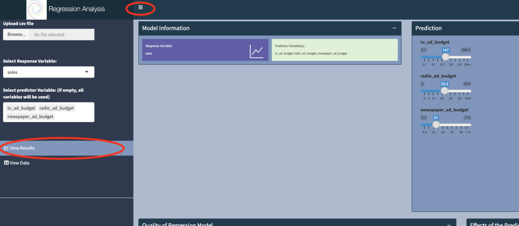
Click on View Results, and toggle the button at the top of the dashboard to obtain optimal viewing.

3. What is the model used

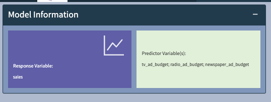
The Model Information panel displays the selection from Step 1, and fits the model of the form:

Sales = a + b*tv_ad_budget + c*radio_ad_budget + d*newspaper_ad_budget

This models says that sales can be determined by a linear combination of tv, radio and newspaper budgets.

4. How to make a prediction

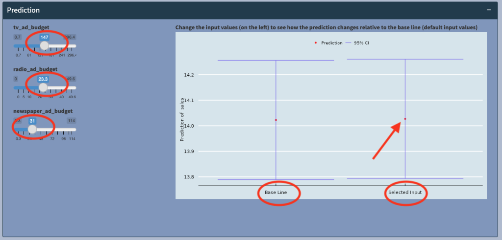
The model will allow us to predict Sales, based on the tv_ad_budget, radio_ad_budget and newspaper_ad_budget information provided in the dataset.

We can look at the effects of these different advertising spending on sales. The plot (above) shows the expected sales (red dot) at the selected input values (147,23.3,31), at around 14.02, with a 95% confidence interval of between 13.75 and 14.4 (blue horizontal bars).

Now if we compare the prediction to the baseline, which is when all the advertising budgets are 0, we see that there is no statistically significantly difference in sales (the two vertical blue bars overlap and are in fact very similar)! that is, at these levels of spending, there’s no significant increase (or decrease) in sales, and the advertising spending was not worth it! 

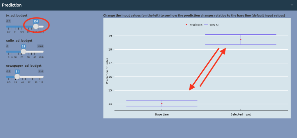
However, when we increase tv_ad_budget to 251, we see that sales increases significantly, and the vertical bars are no longer overlapping! This tells us that at certain, higher levels of spending on TV advertising, sales will significantly increase!

5. What are the effects of the predictors

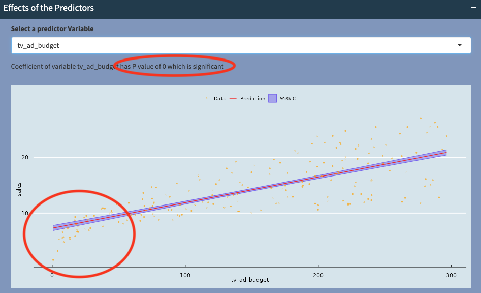
One of the big advantages of the linear regression model is the ability to interpret the effects of the predictors. Here we can see that tv_ad_budget has a positive relationship with Sales (red line with positive incline), and this relationship is statistically very significant (with P-value of 0). The confidence interval bars (purple area around the line of best fit) also tell us how sure we are about this relationship.

Notice that at the bottom left hand corner, the raw data (in orange) appears to fall off the straight line. This could indicate that there is a non-linear relationship between the two variables.

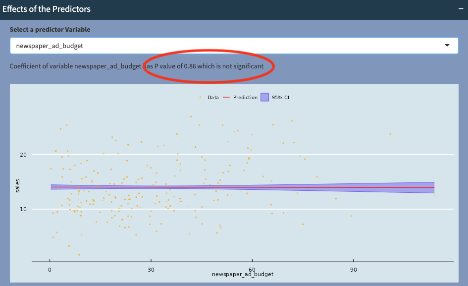
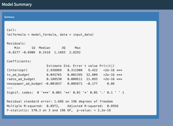
However, when we look at newspaper_ad_budget, we see that the red line is nearly horizontal, so there does not appear to be a strong positive or negative correlation between newspaper_ad_budget and Sales (P-value is 0.86).  We can conclude that newspaper_ad_budget does not contribute significantly towards Sales.

6. How can I tell if the model/prediction is any good?

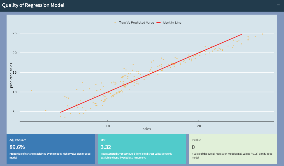
We will want to know how good our model/prediction is, so that we may be able to improve the model (either by adding more/different variables or use a different model).

Here the predicted sales and actual sales values  follow closely to the straight line, indicating that the model is doing a good job.

R squared value of 89.6% indicates a good predictive performance, a P-value of 0 suggests that the variables chosen for this model are good. The mean square error (MSE), is an indication of prediction error. While no model can achieve 0 error, it should be small and can be used to compare models with different variables.

7. What are model assumptions and should I care?

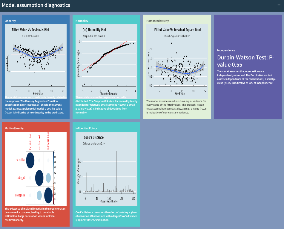
There are several assumptions in the linear regression model. The panel above gives you an indication whether the assumptions have been violated.

In some cases, you shouldn’t sweat too much over mild deviations from assumptions. But severe deviations of many of the assumptions above should be looked at, as these may effect the quality and robustness of your predictions.

For example, if linearity is a problem, you may want a more advanced model to handle non-linear relationships. If normality is an issue, you may want to consider non-parametric regression. If there are outliers, you may want to investigate what causes them.

8. Numerical summary of the regression model

Hopefully you will have everything you need now  to analyse your data. However, if you need more information from the output of the model, we have the output from R, which run the model above.

If you are now ready to give your own dataset a try, follow the link to the